The Results

Run Review

All results can be found in the datalogs folder:

📂working_directory
 ┣ 📂datalogs
 ┃ ┣ 📂51Peg
 ┃ ┃ ┗ 📂run_1
 ┃ ┃ ┃ ┗ 📂k_0
 ┃ ┃ ┃ ┗ 📂k_1
 ┃ ┃ ┃ ┃ ┗ 📂plots
 ┃ ┃ ┃ ┃ ┗ 📂restore
 ┃ ┃ ┃ ┃ ┗ 📂samples
 ┃ ┃ ┃ ┃ ┗ 📂tables
 ┃ ┃ ┃ ┃ ┗ 📂temp
 ┃ ┃ ┃ ┃ ┗ 📜best_fit.dat
 ┃ ┃ ┃ ┃ ┗ 📜log_1_51Peg.dat

The log.dat file contains a summary of the whole run up to this point, plus everything that was printed on the terminal.
The best_fit.dat has a summary of the best values.
The plots folder contains all plots for this run.
The restore folder contains the chain members compressed in .h5 format as well as the residuals of the model. This folder must be targeted to continue a run from this point.
The samples folder is deprecated.
The tables folder contains information about the chains, the parameters and the stats, as well as copy-pastable latex tables.
The temp folder contains all the temporary files made for the run.

Tables

Output example of the latex table, values.tex:

\begin{tabular}{ll}
\toprule
Parameter & Value \\
\midrule
Period 1 & $4.23078861^{+8.2e-06}_{-2.089e-05}$ \\
Amplitude 1 & $55.60434115^{+0.26899442}_{-0.14248269}$ \\
Phase 1 & $1.61264175^{+0.47363979}_{-0.12433487}$ \\
Eccentricity 1 & $0.01221629^{+0.00042225}_{-0.00621666}$ \\
Longitude 1 & $1.11372836^{+0.1321468}_{-0.46498999}$ \\
Acceleration & $-0.00429192^{+0.00011135}_{-0.00028684}$ \\
Offset 1 & $5.21358051^{+0.23550286}_{-0.09804832}$ \\
Jitter 1 & $0.70021693^{+0.15318861}_{-0.45306398}$ \\
\bottomrule
\end{tabular}

Output example of stats.tex:

\begin{tabular}{ll}
\toprule
Stat & Value \\
\midrule
$\log{Z}$ & -902.413 +- 23.211 \\
$\log{P}$ & -859.835 \\
$\log{L}$ & -837.213 \\
BIC  & 1718.787 \\
$chi^{2}_{\nu}$ & 1.035 \\
RMSE & 6.906 \\
\bottomrule
\end{tabular}

the latex table paramter values can be rounded by setting before-hand:

sim.rounder_tables = 3

Plots

Each plot is customisable through its own dictionary. Additionally, you can modify common options through the plot_all property. Every plot has the plot keyword, to turn on or off the plot, as well as a format keyword, default set to 'png'. The plots can be found in the following folders:

📂k_1 ┣ 📂plots ┃ ┗ 📂arviz ┃ ┗ 📂betas ┃ ┗ 📂GMEstimates ┃ ┗ 📂histograms ┃ ┗ 📂models ┃ ┗ 📂posteriors

Posterior Plot

Posteriors are plotted colour-coded by block, in four different formats. To select which modes to plot, include them in the modes list.

Mode	Value (int)	Description
Scatter	0	Simple scatter plot. Useful for checking the overall shape of the posterior distribution.
Hexbin	1	Hexbin plot. Usefull for visualising the samples allocation.
Gaussian filter	2	Scatter plot with markers Gaussian-difussed. Serves both for overall posterior shape and sample density.
Chain	3	A chain plot to oversee the space exploration over time.

Each mode and plotting utility has its own dictionary as well, passed as kwargs to the default matplotlib plotting function. To modify any default values, do it through:

sim.plot_posteriors['modes'] = [0, 3]  # Scatter and chain
sim.plot_posteriors['temps'] = None  # Plots all temperatures. [0, 8] plots for the cold chain and the 8th temp

sim.plot_posteriors['scatter_kwargs']['alpha'] = 0.7  # transparency
sim.plot_posteriors['scatter_kwargs']['s'] = 10  # marker size

sim.plot_posteriors['chain_kwargs']['alpha'] = 0.2  # transparency
sim.plot_posteriors['chain_kwargs']['marker'] = 'o'  # marker shape

sim.plot_posteriors['vlines_kwargs']['alpha'] = 0.75  # global
sim.plot_posteriors['label_kwargs']['fontsize'] = 44  # global

Examples: Posterior plot (mode=0) for the Keplerian Block, cold chain (temp=0): png

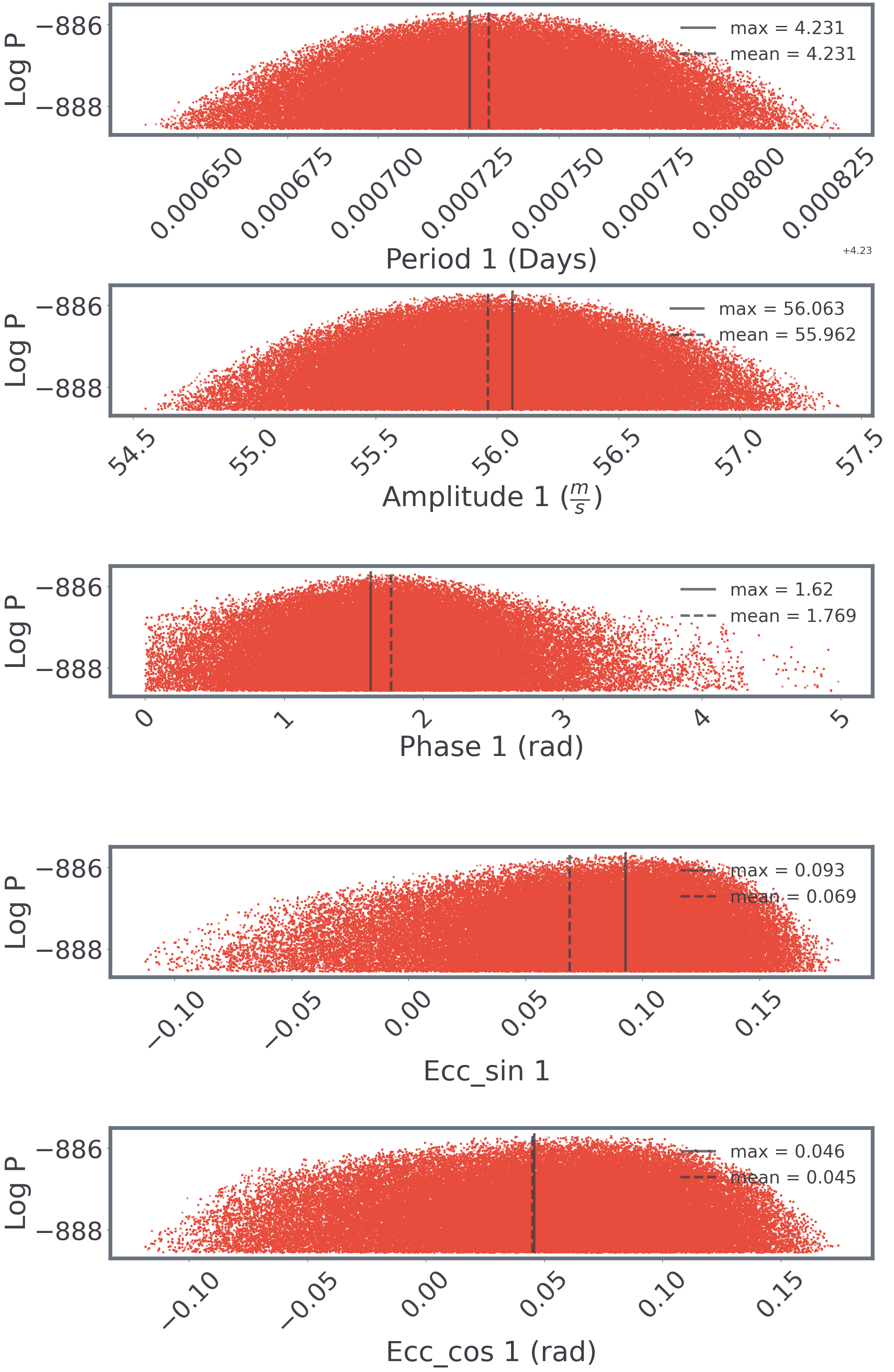
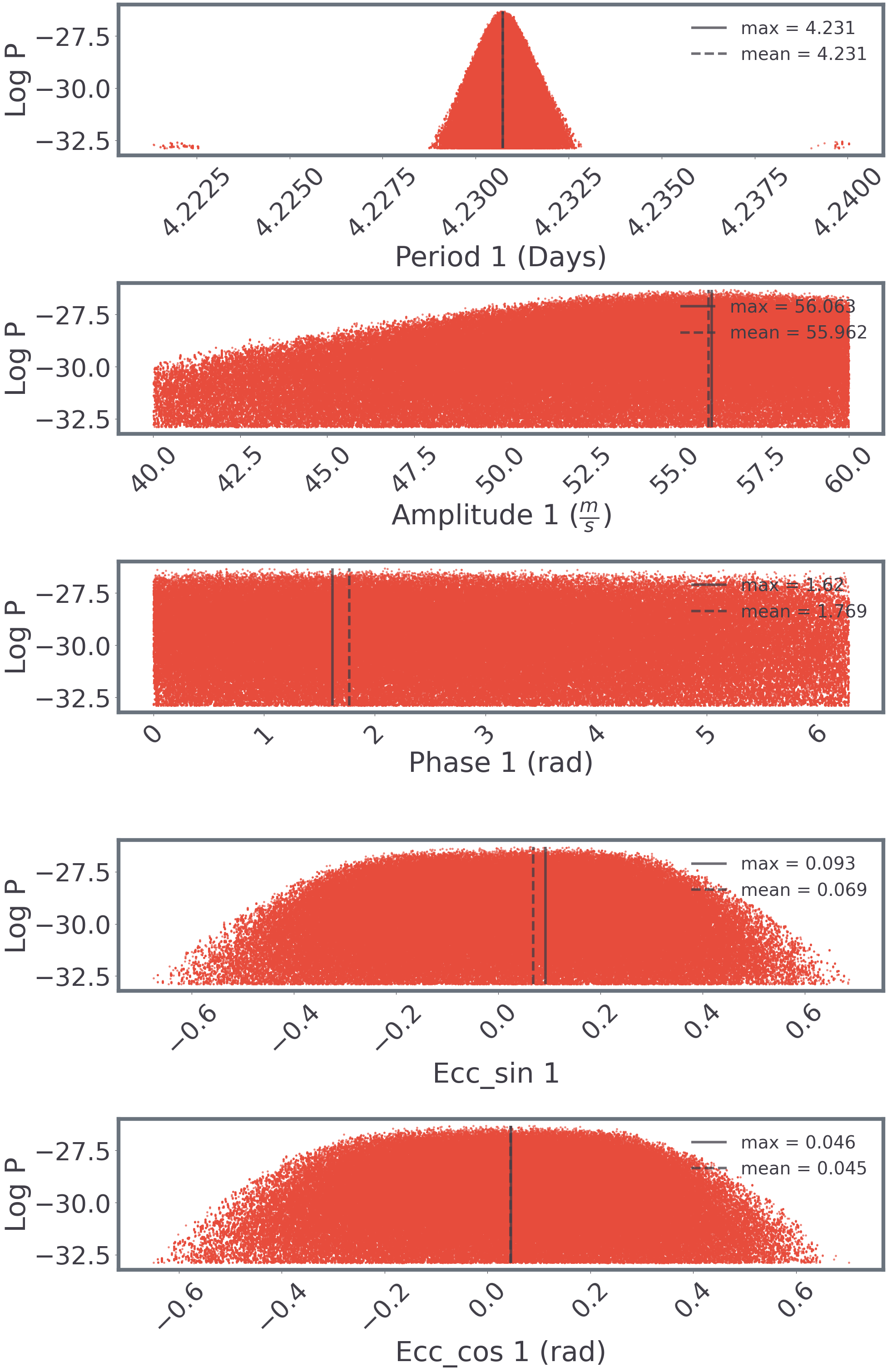
Posterior plot (mode=0) for the same Keplerian Block, at temp=8: png

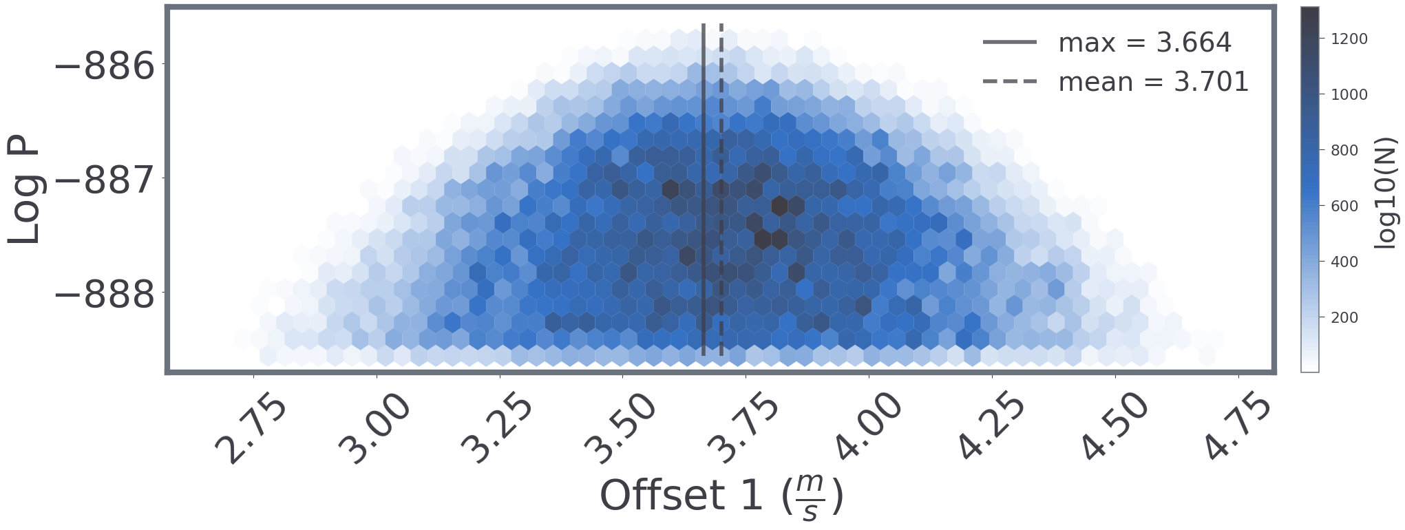
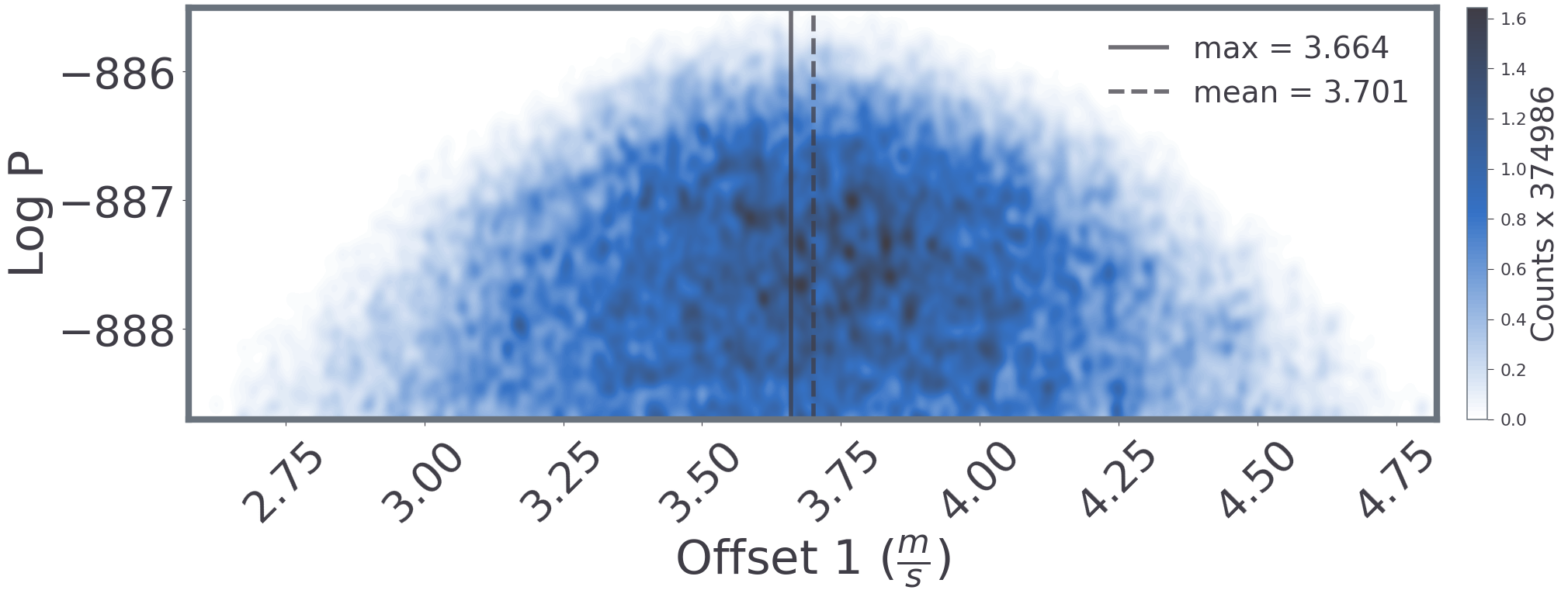
Offset Block, hexbin plot (mode=1): png

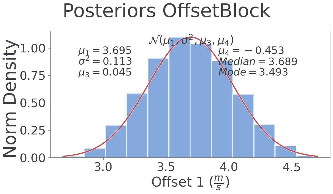
Offset Block, Gaussian plot (mode=2): png

Histograms

sim.plot_histograms['temps'] = None  # Plots all temperatures. [0, 8] plots for the cold chain and the 8th temp

sim.plot_histograms['axis_fs'] = 18
sim.plot_histograms['title_fs'] = 24

Plot of the Histograms:

png

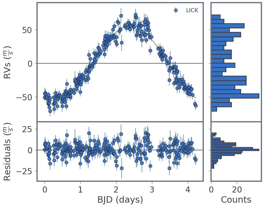
Model

Model with its residuals. Histograms at the side showing the RV distribution.

sim.plot_keplerian_model['hist'] = True  # Turn on/off the histograms

sim.plot_keplerian_model['errors'] = True  # add errorbars for measured error and jitter
sim.plot_keplerian_model['periodogram'] = True  # Plot a periodogram for the residuals

Plot of the Keplerian model: png

Betas

Plots pertaining the reddemcee sampler.

sim.plot_betas['plot'] = True  # Turn on these plots
sim.plot_betas['format'] = 'png'  # save as png

The ladder plot shows the final inverse temperature distribution, against the mean log-likelihood of each chain. Both values are used to estimate the \(\log Z\) with thermodynamic integration: png

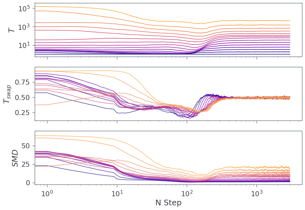
The rate plot helps to assess the adaptation of the temperatures. From top to bottom, temperature evolution over time, temperature swap rate, and Swap Mean Distance: png

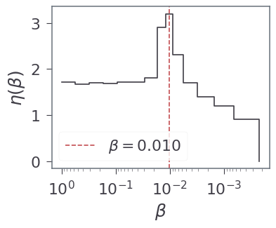
The density plot tracks how close to each other the temperatures are. This is the chain density across temperatures. Peaks signal where phase-change occurs within this MCMC system, or where different solutions merge:

png

Trace Plots

The traceplots are additional plots that require the arviz library installed. Four modes are considered:

Mode	Value (int)
Trace	0
Normalised Posterior	1
Density Interval	2
Corner	3

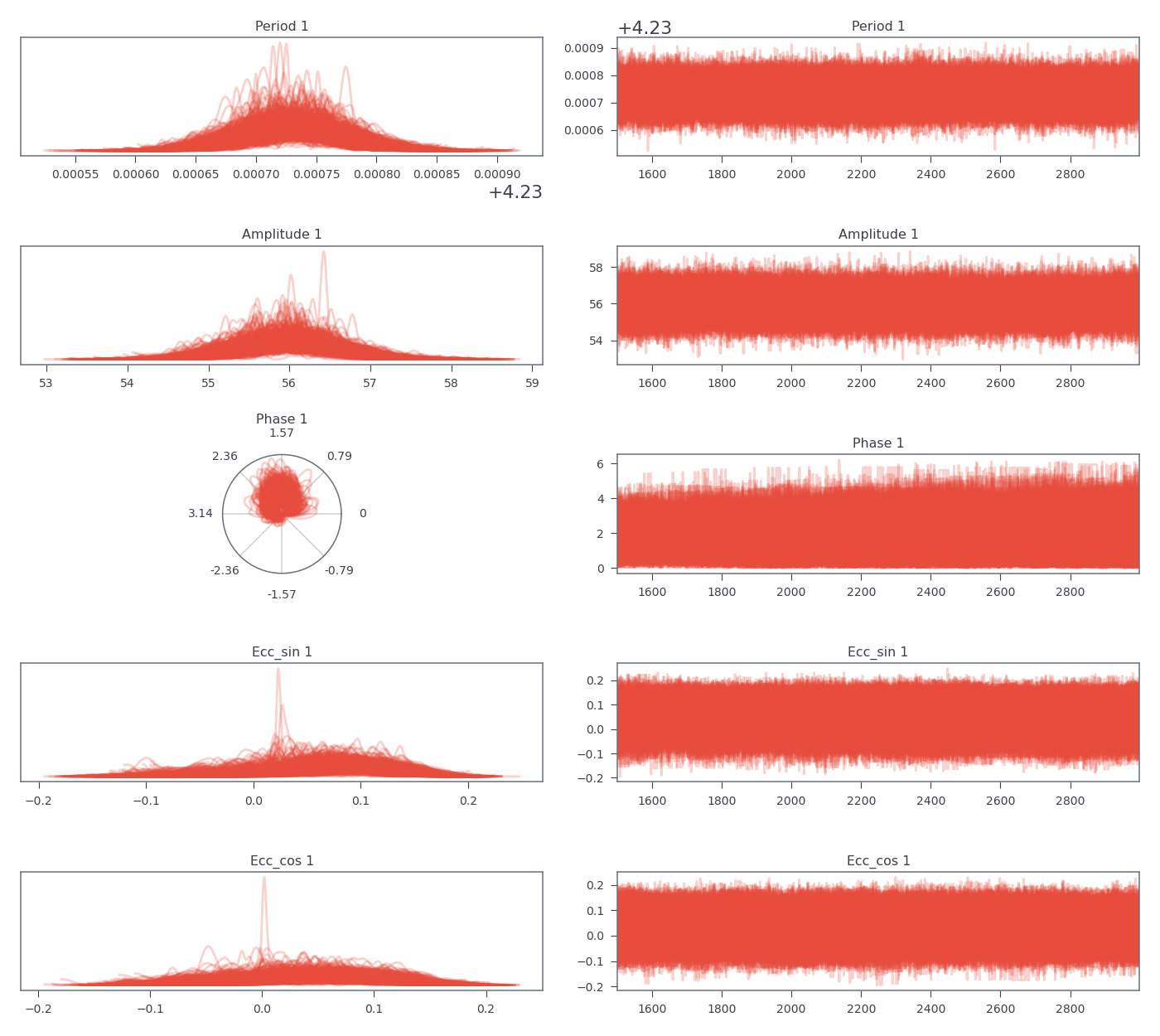
sim.plot_trace['modes'] = [0, 1, 2, 3]

Trace for the Keplerian parameters: png

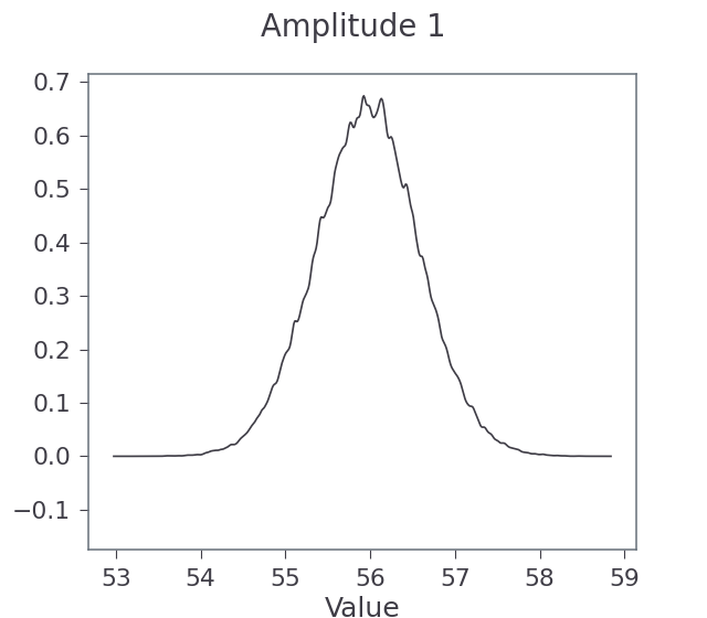
Normalised posterior for the Keplerian amplitude: png

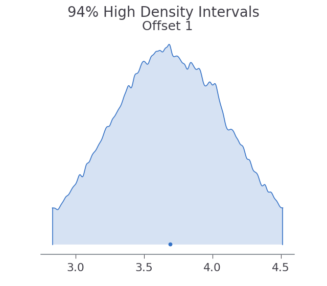
High Density Interval (HDI) for the Offset Block: png

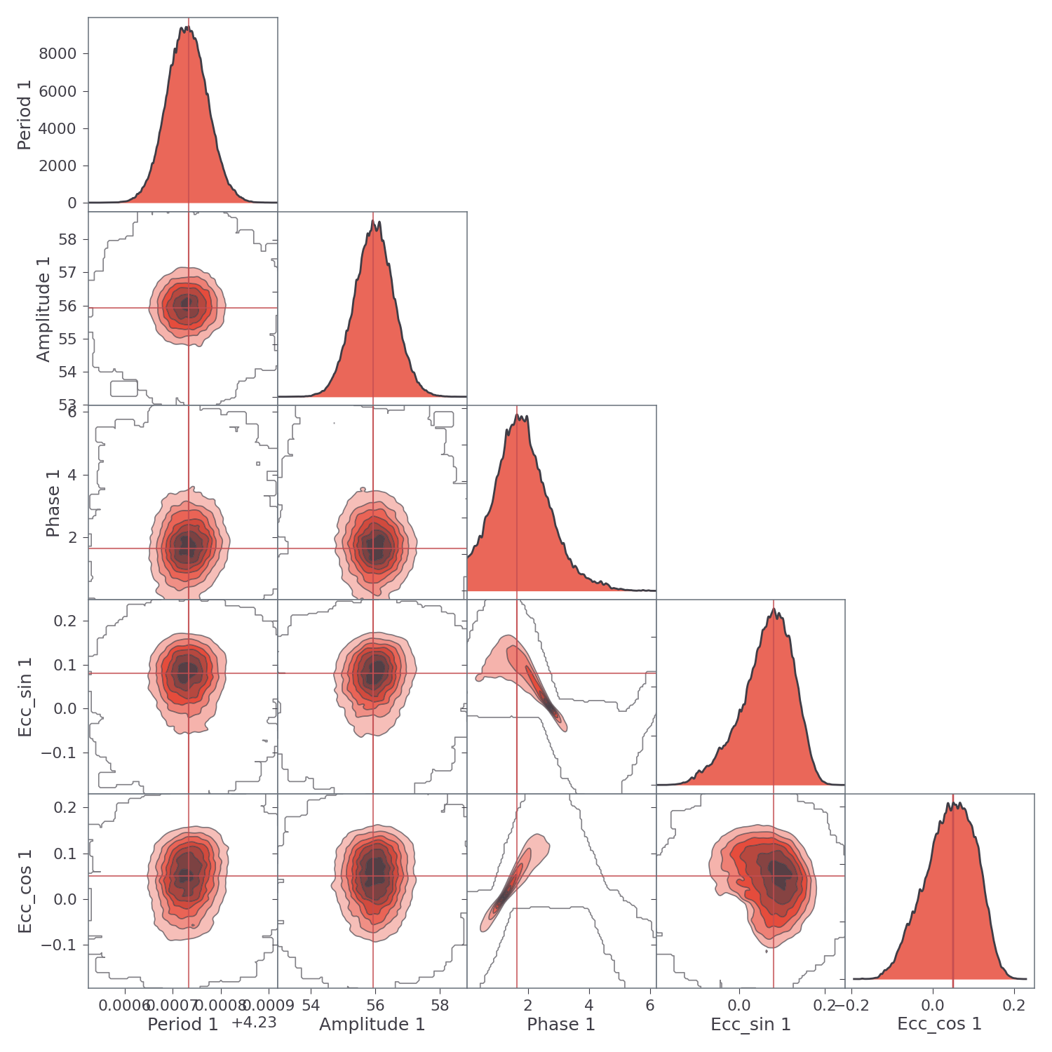
Each Block has its own corner plot, provided it has two or more dimensions. For example, the corner plot for the Keplerian Block: png

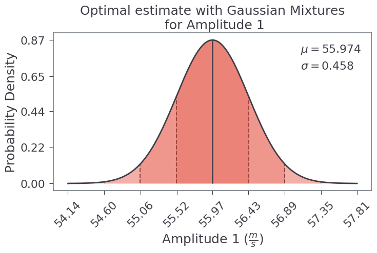
Gaussian Mixtures

The Gaussian Mixtures are also plotted, for example, the amplitude parameter of the Keplerian Block: png